CHAPTER 4 Demand and Supply
Test Yourself
1. (a) The demand curve for a medicine that means life or death for a patient will be vertical, provided the patient has access to any money at all. One would not expect a decline in quantity demanded as the price rises, if that decline meant that the patient would die.
(b) The demand curve for french fries in a food court with many other stands will be fairly flat, perhaps even horizontal. If the firm raises its price at all, many if not most of its customers will just move to a different stand. Thus a small change in price results in a large change in the amount of fries bought.
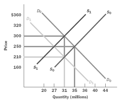
3. The answers to all three parts are shown in Figure 2.
(a) Initially, the equilibrium price is $250, and the equilibrium quantity is 35 million bicycles, as shown by the intersection of D0 and S0.
(b) If demand falls by 8 million bikes per year, the new demand curve is D1. The price falls to $210, and the quantity falls to 31 million, as shown by the intersection of D1 and S0. Although demand falls by 8 million at each price, the quantity exchanged falls by only 4 million because the price fall has induced a movement out along the new demand curve, as well as a movement back along the old supply curve.
(c) If supply falls by 8 million bikes per year, the new supply curve is S1. The price rises to $300, and the quantity falls to 31 million, as shown by the intersection of D0 and S1. Although supply falls by 8 million at each price, the quantity exchanged falls by only 4 million because the price increase has induced a movement out along the new supply curve, as well as a movement back along the old demand curve.
(d) If demand and supply each fall by 8 million bikes per year, the equilibrium price is $250, and the equilibrium quantity is 27 million bicycles, as shown by the intersection of D1 and S1.
Figure 2

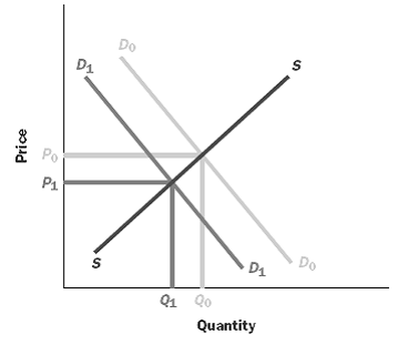
5. The same diagram, Figure 4, can be used for all three cases, because they all entail a decline in demand, from D0 to D1. Price falls from P0 to P1, and quantity falls from Q0 to Q1.
(a) In a drought, people have less need for umbrellas, so demand falls.
(b) Popcorn is a complement for movie tickets, so when popcorn prices rise, the demand for tickets falls.
(c) Coca-Cola is a substitute for coffee, so when the price of the soda falls, the demand for coffee falls.
Figure 4
8. (a) With a 50-cent tax per pound of beef, Table 2 in the text must be adjusted:
Price Paid by
Consumers Price Received by Farmers Quantity Supplied
(dollars per pound) (dollars per
pound) (pounds per year)
8.00 7.50 90
7.90 7.40 80
7.80 7.30 70
7.70 7.20 60
7.60 7.10 50
7.50 7.00 40
7.40 6.90 30
(b) Using the new Table 4-2, Figure 6 shows that the new supply curve, S1 lies above the original curve, S0, by a distance of 50 cents at each output. The new equilibrium price is approximately $7.76, and the new equilibrium quantity is approximately 47 pounds.
Figure 6
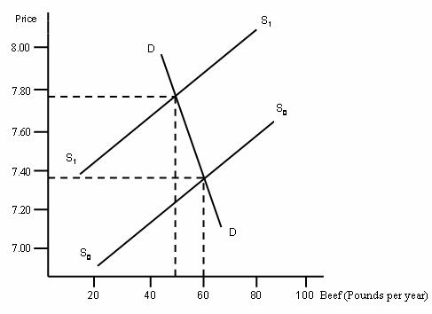
(c) Yes, beef consumption falls by approximately 13 pounds.
(d) The equilibrium price rises by approximately 36 cents, which is less than the tax.
(e) Consumers pay two thirds of the tax, since the price they pay has risen by 36 cents.
Producers pay one third, since the price they receive has fallen.
Discussion Questions
1. This question is intended to help students develop an intuitive sense of the origins of the demand curve. If you deal with this question in class or discussion section, it will be revealing to aggregate the students’ answers, and derive a “market” demand curve. It is also interesting to see whose purchases are sensitive to the price increase, and whose are not, and to speculate upon the reasons for the difference.
4. In Figure 8 (a), the equilibrium price of milk is PE. The government wishes to raise the price to PF, and it therefore pays farmers to slaughter cattle. As a consequence, the supply curve falls to S1 and the price rises. The market for meat is shown in (b), where the added slaughters increase the supply to S1, cut the price to P1 and raise the quantity to Q1.
Figure 8

5. Figure 9 shows three different prices. P1 is an effective price ceiling, at which the quantity demanded, G, exceeds the quantity supplied, F. P2 is the equilibrium price, at which the quantity supplied and the quantity demanded are equal, at E. P3 is an effective price floor, at which the quantity supplied, I, exceeds the quantity demanded, H. Consider first the price ceiling, P1. Since supply curves are positively sloped, at this price the quantity supplied must be less than at the equilibrium P2. And since sellers cannot be forced to sell any more than they wish, the quantity exchanged will be F, which is lower than the equilibrium quantity E, in spite of the fact that buyers wish to buy more, G. Consider next the price floor, P3. Since demand curves are negatively sloped, the quantity demanded at this high price will be less than the quantity demanded at the equilibrium. Since buyers cannot be forced to buy more than they want, the quantity exchanged at this price is H, which is less than the equilibrium quantity E. These results follow from the common-sense observation that exchange is voluntary. At any price above or below the market equilibrium price, the quantity exchanged is less than it would be at the equilibrium.
Figure 9

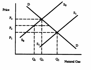
8. The congressman was confused. Figure 11 shows the market for natural gas. If the supply curve is S0 and the demand curve D, then the equilibrium price is Pe, and the equilibrium quantity Qe. But a price ceiling of Pc has reduced the quantity sold to Qc. If the ceiling is removed, the quantity produced rises to Qe, but this increase is a market response to the increased price. The congressman has confused a movement along the supply curve with an increase in supply, which would be shown by a new supply curve S1, and which would indeed bring the price down to P1. But there is no reason to think that removal of the price ceiling will lead to such a shift in the supply curve. This is true even if new firms enter the market. Any increase in production induced by an increase in price (whether from existing firms or from new firms) is represented by a movement along the supply curve. A shift in supply occurs only when some factor other than price changes.
Figure 11
9. Explanation (b) is more consistent with the data. If the principal change in the market had been an increase in supply of female workers, i.e., explanation (a), then female wages would have fallen. The fact that they increased while employment also increased means that demand for female workers must have grown.